This lecture introduces the GLove model, the intuition behind the algorithm and different means to evaluate them.
Glove was an algorithm for word vectors that was made by Jeffrey Pennington, Richard Socher, and Christopher Manning in 2014 and acted as the starting point of connecting together the linear algebra based methods on co-occurrence matrices like LSA and COALS with the models like skip-gram, CBOW and others, which were iterative neural updating algorithms. The earlier linear algebra methods actually had their advantages for fast training and efficient usage of statistics, the results weren’t as good perhaps because of disproportionate importance given to large counts in the main. Conversely, the neural models seemed to performing gradient updates on word-windows, and inefficiently using statistics versus the co-occurrence matrix. Though, it was actually easier to scale to a very large corpus by trading time for space.

The motivation was to use neural methods, which generated improved performance on many taskss, and identify the properties necessary to have these analogies work, such as going from male to female, queen to king. Or going from a verb to its agent, truck to driver.
Analogies and Meaning components
The intent behind the Glove design was to represent the “meaning” components as ratios of co-occurrence probabilities. As an example, the below illustrates the spectrum from solid to gas as in physics. The word “solid” co-occurs with the word “ice” often, while the word “gas” doesn’t occur with the word “ice” as many times. But the problem is the word “water” will also occur a lot with ice, while any other random word like the word “fashon”, doesn’t occur with the word “ice” many times. In contrast, if we look at words co-occurring with the word “steam”, “solid” won’t occur with “steam” many times, but “gas” will. The water will also co-occur again and “fashion” occurence will be small. So to determine the meaning component of traversing from gas to solid, it would be useful to look at the ratio of these co-occurrence probabilities.
Because then we get a spectrum from large to small between solid and gas. Whereas for water and a random word, it basically cancels out and gives youI just wrote these numbers in.

In an actual large corpus, the following are actual co-occurrence probabilities.
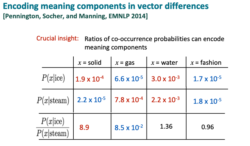
as noted the co-occurence probabilities cancel out for “water” and while for fashion is it low, both around 1. Whereas the ratio of probability of co-occurrence of solid with ice or steam is about 10. And for gas it’s about a 10th.
Log bi-linear model
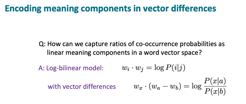
In order to capture these ratios of co-occurrence probabilities as linear meaning components within the word vector space, we can just add and subtract linear meaning components. This can be achieved using a log-bilinear model. So that the dot product between two word vectors attempts to approximate the log of the probability of co-occurrence. So if you do that, you then get this property that the difference between two vectors, its similarity to another word corresponds to the log of the probability ratio shown on the previous figure.
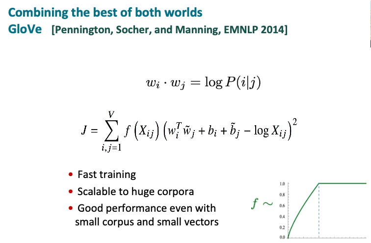
So the GloVe model attempts to unify the thinking between the co-occurrence matrix models and the neural models by being some way similar to a neural model 1. calculated on top of a co-occurrence matrix count. 2. Has an explicit loss function.
And the explicit loss function is the diference of the dot product to the log of the co-occurrence. To prevent very common words from dominating, the effect of high word counts are capped using the f function. This structure allows the optimization of the J function directly on the co-occurrence count matrix, providing a fast training scalable to huge corpora.
Objective function for the GloVe model / log-bilinear means
log-bilinear - the “bi” is indicative of the two terms wi and wj, similar to an algebraic value of ax where the term i linear in x and a is a constant. The difference is squared to ensure that the term is always positive and J is a minimization problem. There are two bias terms for both words which can move things up and down for the word in general. So if in general probabilities are high for a certain word, this bias term can model specifically for that word.
Explanation for f(Xij)
f(Xij) is provided to scale things depending on the frequency of a word because we want to pay more attention to words that are more common or word pairs that are more common. But there is a potential issue when we have extremely common words like function words. So the function f(Xij) typically pays attention to words that co-occurred together up until a certain point. And then the curve just goes flat, so it didn’t matter if it was even an extremely, extremely common word.
Results
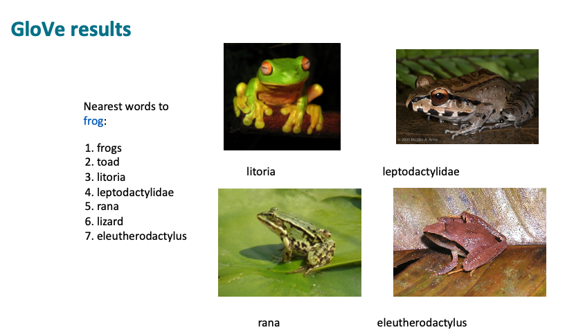
Nearest words to the word “frog” - We get “frogs”, “toad”, and then we get some complicated words. But it turns out they are all frogs,u ntil we get down to lizards.
Evaluation of Glove algorithm
There are typically two ways of evaluation - Intrinsic and extrinsic. In an intrinsic evaluation we evaluate directly on the specific or intermediate subtasks that we’ve been working on. Intrinsic evaluations are fast to compute and help understand the component we’ve been working on.
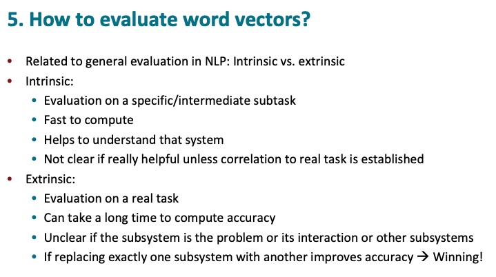
An extrinsic evaluation is to utilize a real task of interest, such as web search or machine translation and use that goal to improve performance on that task. However, such evaluation takes longer due to the extensiveness of the system involved. And sometimes it is difficult to attribute the result to the appropriateness of the word vectors or due to some other components of the system or if the interaction was just better with your previous version of the word vectors.
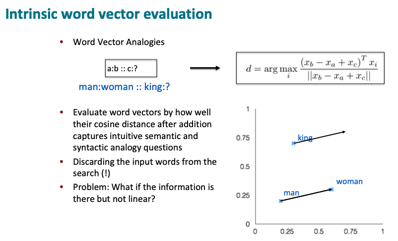
For intrinsic evaluation of word vectors, we can provide models with a big collection of word vector analogy problems, such as man is to woman as king is to blank? And tune the model to find the word that is closest, such as queen and produce an accuracy score of how often that the model evaluates it accurately.
Note: Many times during such evaluation, the actual closest word is really just “king”. So to prevent this issue, the three input words are not allowed in the selection process, choosing only the nearest word that isn’t one of the input words.
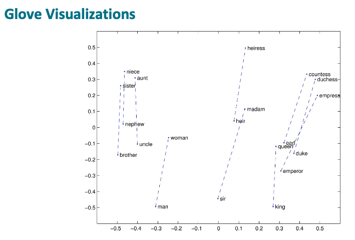
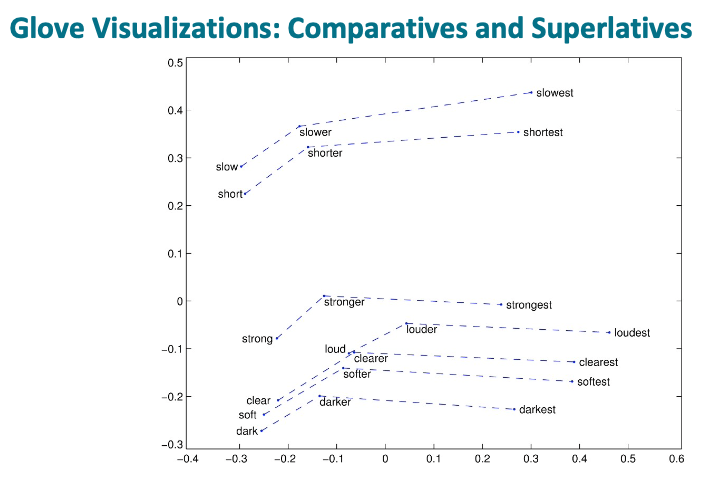
From the GloVe vector examples above, they exhibit a strong linear component property such as the male-female dimension. For example, taking the vector difference of “man” and “woman” and adding the vector difference onto “brother”, the expectation is to get to “sister” and king, queen, and for many of these examples. But some examples may not work, such as starting from “emperor”, the vector might get to “countess” or “duchess” instead.
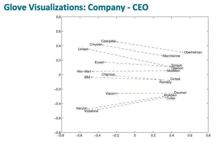
And these two examples illustrate that the Company to CEO and superlatives also move in roughly linear components.
Evaluation Metrics
word2vec authors built a data set of analogies to evaluate different models on the accuracy of their analogies, including semantic and syntactic analogies. Unscaled co-occurrence counts via an SVD work terribly. Some scaling can get SVD of a scaled count matrix to work reasonably well, hence SVD-L is similar to the COALS model. They do a decent enough job without a neural network.

The results also illustrate how word2vec and GloVe models performed and in 2014 was considered optimal. However, it might have scored better due to better data.
Better Data
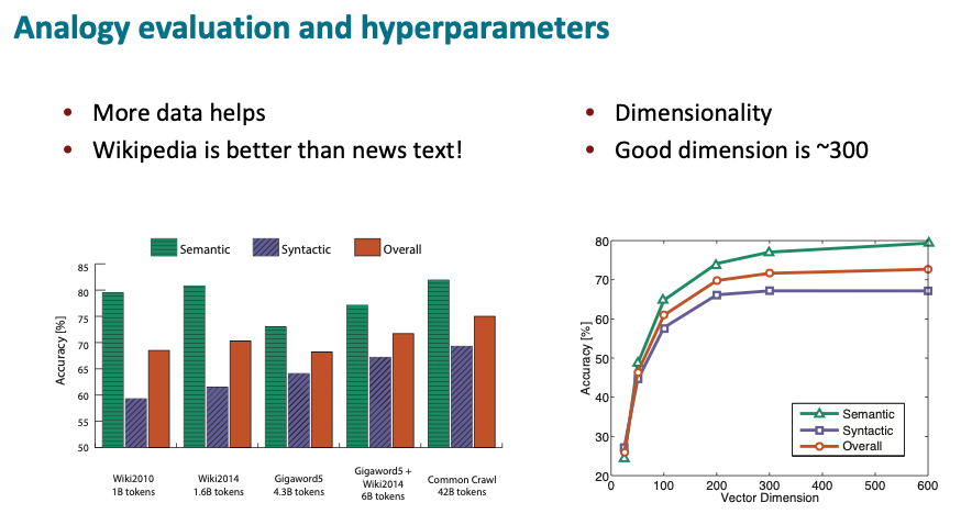
The above image illustrates the semantic, syntactic and overall performance on word analogies of GloVe modelthat when trained on different subsets of data. One of the big advantage was that the GloVe model was partly trained on Wikipedia as well as other text. Whereas the word2vec model that was released was trained exclusively on Google News, which is not as good as even one quarter of the size amount of Wikipedia data for semantics. On the right end, with Common Crawl Web data, 42 billion words, we get good scores again from the semantic side.
The graph on the right then shows performance against the vector dimension. 25 dimensional vectors score poorly, while 100 dimensional vectors already work reasonably well, but still get significant gains for 200 and somewhat to 300 and recently 300 dimensional vectors seems to be the sweet spot, with the best known sets of word vectors, including the word2vec vectors and the GloVe vectors provide 300 dimensional word vectors.
Human judgments of word similarity
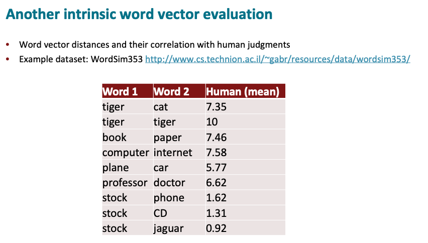
Another intrinsic evaluation you can do is see how these models model human judgments of word similarity. So psychologists for several decades have actually taken human judgments of word similarity. Where literally you’re asking people for pairs of words like “professor” and “doctor” to give them a similarity score that’s being measured as some continuous quantity giving you a score between, say 0 and 10.
They responses are then averaged over multiple human judgments as to how similar different words are. For example, “tiger” and “cat” are pretty similar. “Computer” and “internet” are pretty similar, while “Plane” and “cars” less similar. “Stock” and “CD” aren’t very similar at all but “stock” and “jaguar” are even less similar.

And in particular, we can measure a correlation coefficient of whether they give the same ordering of similarity judgments. And there are various different data sets of word similarities and scorinf of different models as to how well they do on such similarities. Plain SVD’s works comparatively better here for similarities than it did for analogies, not completely terrible because we no longer need that linear property. Scaled SVD’s work a lot better, Word2vec works a bit better than that and with similar minor advantages from the GloVe model.
Extrinisic Evaluation
NER (named entity recognition) is an extrinsic task for identifying
mentions of a person’s name or an organization name like a company or a
location. Having good word vectors help perform named entity recognition
effectively. Starting with a model with discrete features, which uses
word identity as features, we can build a named entity model doing that
and adding word vectors provides a better representation of the meaning
of words. 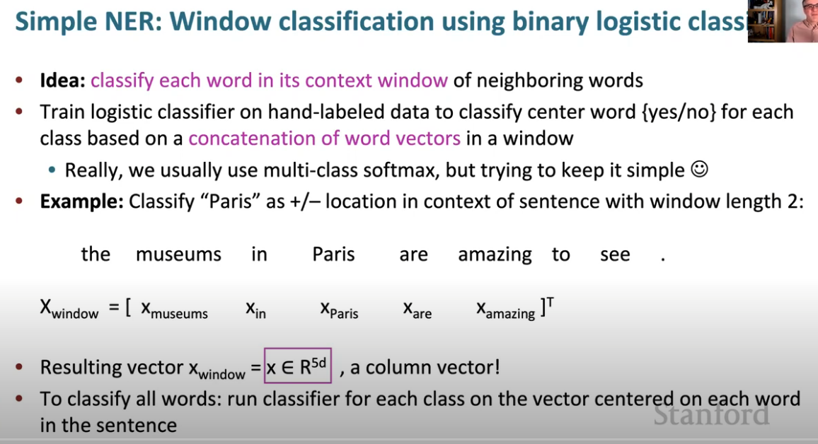
On the Intrinsic and Extrinsic Fairness Evaluation Metrics for Contextualized Language Representations by Yang Trista Cao et al. is a good reference on these different evaluation metrics and underlying biases.
Word Senses and word sense ambiguity
There are different meanings of the word pike
- A sharp point or staff
- A type of elongated fish
- A railroad line or system
- A type of road
- The future (coming down the pike)
- A type of body position (as in diving)
- To kill or pierce with a pike
- To make one’s way (pike along)
- In Australian English, pike means to pull out from doing something: I reckon he could have climbed that cliff, but he piked!
Improving Word Representations Via Global Context And Multiple Word Prototypes (Huang et al. 2012)
The gut feeling is usually to have different vectors for each meaning of the same word, as it seems counter-intutive to have the same vector for all the different meanings. If “Pike”, and other words have “word sense” vectors. This paper attempted to improve the representation of words such as “pike”. The primary idea was to cluster word windows around words, retrain with each word assigned to multiple different clusters bank1, bank2, etc. And then for the clusters of word tokens, start treating them as if they were separate words and learning a word vector for each. So basically this does work and we can learn word vectors for different senses of a word. But actually this isn’t the majority way that things have then gone in practice. Primarily due to increased complexity, and it tends to be imperfect in its own way as we’re trying to take all the uses of the word “pike” and sort of cut them up into key different senses, where differences overlap and there is no clear distinction. It’s always very unclear how you cut word meaning into different senses.
In an overall sense, the word vector is generated as a superposition of the word vectors for the different senses of a word, here “superposition” means no more or less a weighted sum. So the vector that we learn for “pike” will be a weighted average of the vectors that would have learned for the medieval weapons sense, plus the fish sense, plus the road sense, plus whatever other senses that you have, where the weighting that’s given to these different sense vectors corresponds to the frequencies of use of the different senses.
And adding up several different vectors into an average does not lose the real meanings of the word and it turns out that this average vector in applications, tends to self-disambiguate.
References
Suggested Readings
- GloVe: Global Vectors for Word Representation (original GloVe paper)
- Improving Distributional Similarity with Lessons Learned from Word Embeddings
- Evaluation methods for unsupervised word embeddings