This blog post captures the inner workings of the Word2Vec Algorithm, by roughly following the lecture patterns for the Cs224n course from Stanford.
Word2vec algorithm
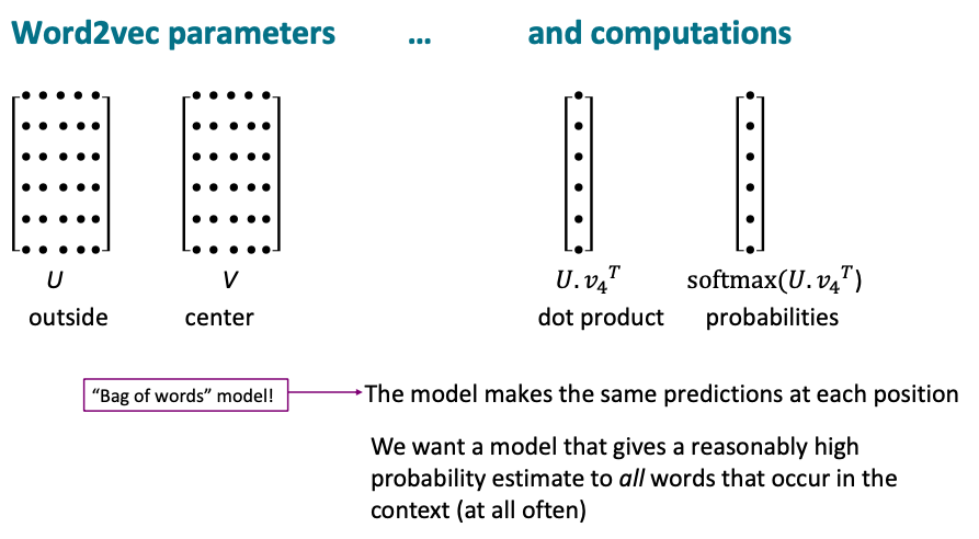
Recalling the Word2vec algorithm from Introduction-to-nlp-and-word-vectors, the only parameters of this model are the word vectors. We have context word vectors and center word vectors for each word and then taking their dot product to get a probability, which gives a score of how likely a particular context word is to occur with the center word. Using the softmax transformation on the dot product converts the scores into probabilities. word2vec model is called a bag of words (BoW) model. BoW models does not pay any attention to word order or position, the distance of the context words from the center word while computing the probability estimate.
Optimization: Gradient Descent
The next step would be to determine the gradient of the loss function with respect to the parameters. The algorithm starts with random word vectors. They are initialized with small numbers, near 0 in each dimension. The loss function J uses a gradient descent algorithm, an iterative algorithm, that learns to maximize J(θ) by changing theta, which represents the model weights. The idea of the algorithm is to calculate the gradient J(θ), from the current values of θ, by making a small step in the direction of the negative gradient to gradually move down towards the minimum.
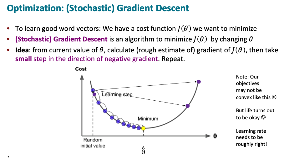
The simple gradient descent works the following way: The step size parameter of the algorithm determine the time taken and if the function converges. If the step size is too smal, it would take a long time to minimize the function while a large step can make the function diverge and keep getting bouncing back and forth. The algorithm steps a little bit in the negative direction of the gradient using the step size, which gives new parameter values. But ach individual parameter gets updated only a little bit by working out the partial derivative of J with respect to that parameter and by using the learning rate, where J is a function of all windows in the corpus.
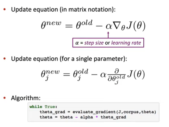
Note that the denominator is a sum over every center word in the entire corpus, but they often have billions of words in the corpus, which makes computing the gradient of J(θ) expensive, as we have to iterate over the entire corpus. So a single gradient update takes a long time and optimization would be extremely slow.
Stochastic Gradient Descent
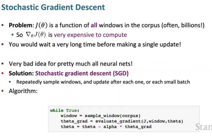
The alternative to avoid the above issue is to use stochastic gradient descent. So rather than working out an estimate of the gradient based on the entire corpus, we take one center word or a small batch of 32 center words, work out an estimate of the gradient based on them. Now that estimate of the gradient will be noisy and bad because only a small fraction of the corpus was used rather than the whole corpus. But nevertheless, we can use that estimate of the gradient to update the theta parameters in exactly the same way. So with a billion word corpus, with each center word, we can make a billion updates to the parameters as we pass through the corpus once rather than only making one more accurate update to the parameters using the entire corpus. So overall, we can learn several orders of magnitude more quickly.
Neural nets have some quite counter intuitive properties and even though the stochastic gradient descent is noisy and bounces around, the complex networks learns better solutions than when using a plain and slow gradient descent.
Note about SGD
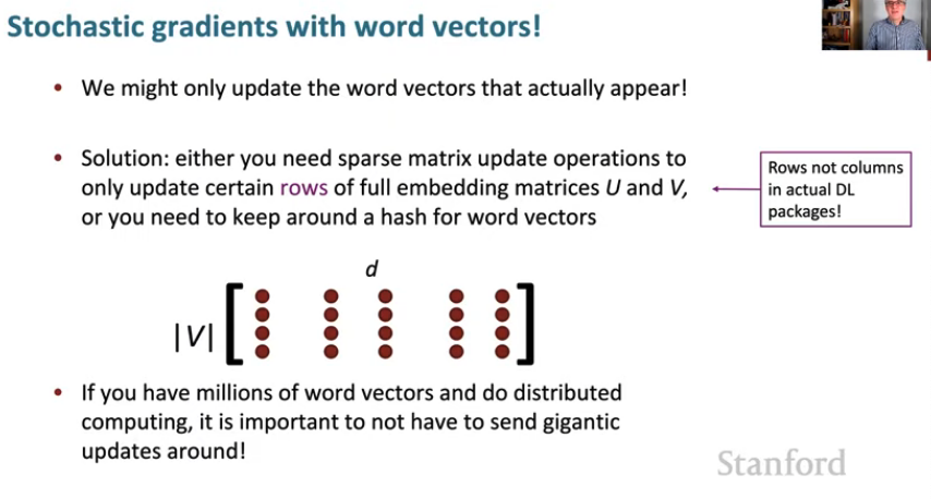
For example, when performing stochastic gradient update for one window, with one center word and window size of 5, there would be at most 11 distinct word types. So gradient information will be available for those 11 words but the other 100,000 words in our vocabulary will have no gradient update information, making it a very sparse gradient update. Thinking from a systems optimization perspective, we would ideally want to update the parameters only for a few words and there are many efficient ways to achieve that.
Note: word vectors have been presented as column vectors, which is usually how mathematical notation prescribes, however in deep learning packages, word vectors are actually represented as row vectors
Why two different vectors for the same word
If we use the same vector for context and center, and if the same word occurs in the same window as both a center and a context word, then a dot product of the same term with itself, makes it messier to work out.
Word2Vec model functions
word2vec can operate in two different models 1. skip-gram model - where it predicts the context words given the center word in a bag of words style model. 2. Continuous Bag of Words model - where it predicts the center word from a bag of context words.
The original word2vec paper used the skip-gram model and used negative sampling also called SGNs (skip-grams negative sampling), instead of the naive softmax. This was due to the expensive cost of computing the denominator you have to iterate over every word in the vocabulary and work out these dot products for every word in the corpus for each window. While negative sampling trains binary logistic regression models for both the true pair of center word and the context word versus noise pairs where the true center word and randomly sample words from the vocabulary are paired, and updates only the related weights, instead of updating all of the weights.
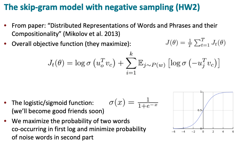
Instead of softmax, the dot product is passed through the logistic function (sigmoid), which maps any real number to a probability between 0 and 1 open interval. So for a large dot product. the logistic function would return 1.
On average the dot product between the center word and context words, should be small if they most likely didn’t actually occur in the context. This is achieved using the sigmoid function, which is symmetric and to make probability small, we can take the negative of the dot product i.e., The dot product of a random context word and the center word would be a small number, which is again negated to put through the sigmoid.
The objective is to actually maximize the Jt(θ).
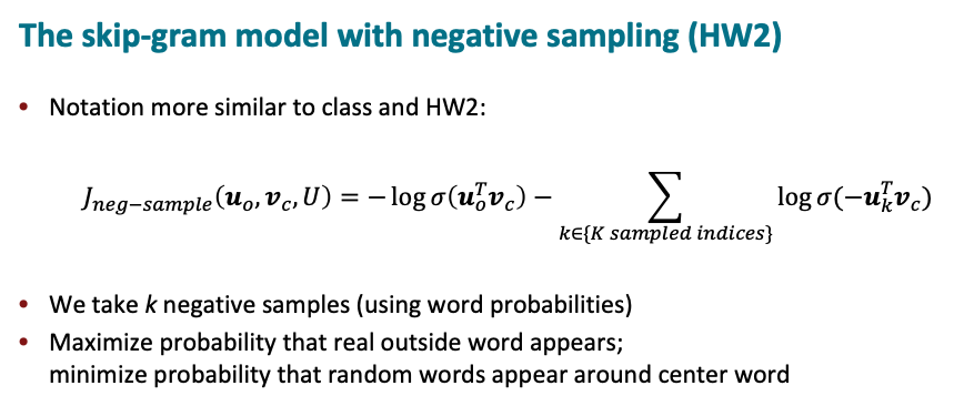
Comparing this to the earlier discussion of minimizing the negative log likelihood, where we use the negative log likelihood of the sigmoid of the dot product and use k-negative samples of random words. This loss function would be minimized given this negation of the log of the dot product ,by making these dot products large, and the small k-negative dot products are negated which would be small postive after going through the sigmoid.
Better sampling of rare words
While sampling, the authors of the word2vec sample the words based on their probability of occurrence using the unigram distribution of words, which defines how often words actually occur in the corpus. For example, in a billion word corpus, a particular word occurred 90 times in it, the 90 divided by a billion, is the unigram probability of the word. It is also (3/4)th powered, which renormalizes the probability distribution and dampens the difference between common and rare words to ensure that less frequent words are sampled more often, but still not nearly as much as if a uniform distribution was utilized.
Problems with co-occurence matrix
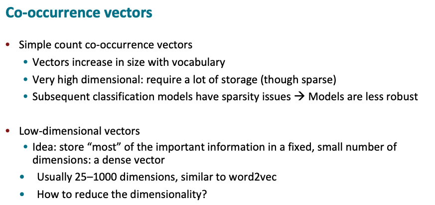
- Cooccurence matrices are huge very sparse For example with vocabulary of half a million words, we have half a million dimensional vector.
- Results tend to be noisier and less robust depending on what words are available in the corpus.
- So for better results we should work with low dimensional vectors.
- In practice the dimensionality of the vectors that are used are normally somewhere between 25 and 1,000.
Singular Value Decomposition
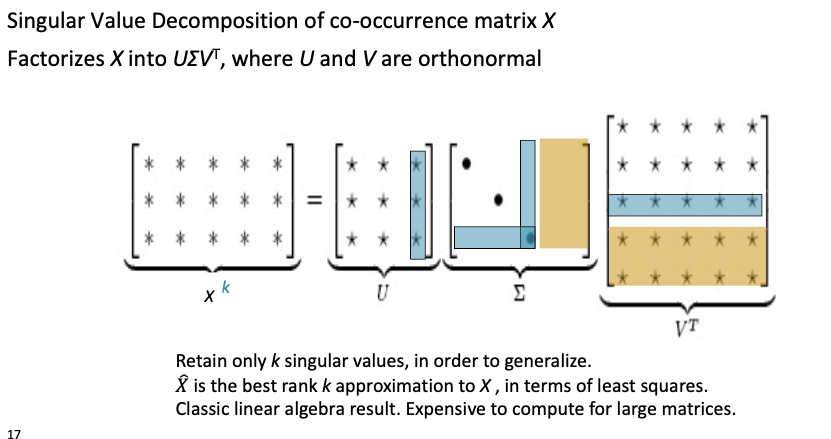
Singular value projection gives an optimal way under a certain definition of optimality, of producing a reduced dimensionality pair of matrices that maximally recovers the original matrix. So the cooccurence count matrix can be decomposed into three matrices - a diagonal matrix U, sigma, and a V transpose matrix. We can take advantage of the fact that the singular values inside the diagonal sigma matrix are ordered from largest down to smallest and discounting some of the smaller values, we can extract lower dimensional representations for our words which enables us to recover the original co-occurrence matrix. But it works poorly because we are expecting to have these normally distributed errors because we have exceedingly common words like “a,” “the,” and “and” and a very large number of rare words.
We can use the log of the raw counts or cap the maximum count or remove the function words to address this issue and such methods were explored heavily in the 2000s.
COALS
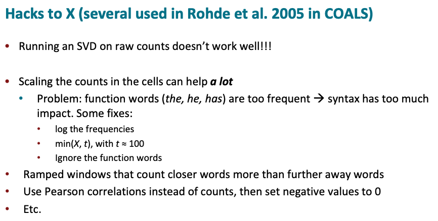
Doug Rohde explored a number of these ideas as to how to improve the co-occurrence matrix in a model that he built that was called COALS. We get the same kind of linear semantic components, which can be used to identify analogies.
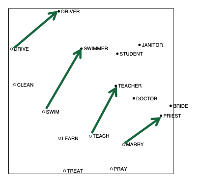
These vector components are not perfect, but are roughly parallel and roughly the same size. And so we have a meaning component there that we could add on to another word for analogies. We could determine drive is to driver as marry is to a priest. This acted as the basis for the Glove model investigation.